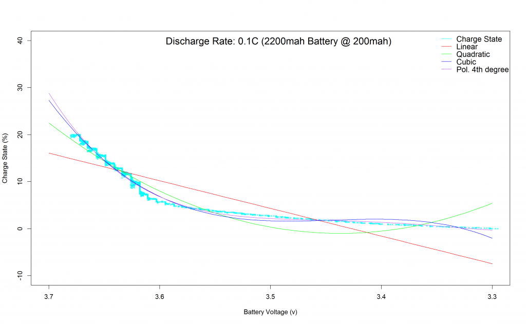
Estimating the state of charge of a lithium based on voltage measurements from the battery is rather challenging. This is due to not only the state of chacrge but also the condition of the battery, current drawn, ambient temperature, etc all having a significant impact on the voltage measured. The best way for SoC estimation would be a columb counter which wasn’t available for my project. For my project the current drawn is rather constant around 200ma and the temperature is relatively stable around 20-25C. Thus a much better estimate should be possible with polynomials than the simple linear SoC estimations. For the polynomial regeressions and to find the polynomial coefficients r was used.

For the data a 2200mah battery from Seeedstudio was discharged at 200ma with an iCharger 106i+. Interestingly the capacity of the battery was found to be exactly 2200mah which speaks for the quality of seedstudios batteries. The resulting datalog can be downloaded at the bottom of this post.

R Code for the polynomial regressions:

stats <- readWorksheet(loadWorkbook('C:/Project Details/stats.xlsx'),sheet=1)
y <-  stats[,"Charge"]
x <-  stats[,"Voltage"]
fit1 <- lm(y~x)
fit2 <- lm(y~poly(x,2,raw=TRUE))
fit3 <- lm(y~poly(x,3,raw=TRUE))
fit4 <- lm(y~poly(x,4,raw=TRUE))
xx <- seq(3.3,4.20, length=50)
plot(x,y,pch=4, col=69, cex=0.5, xlim=c(4.25,3.2),ylim=c(-10,100), type="p", ylab='Charge State (%)',xlab='Battery Voltage (v)')
lines(xx, predict(fit1, data.frame(x=xx)), col="red")
lines(xx, predict(fit2, data.frame(x=xx)), col="green")
lines(xx, predict(fit3, data.frame(x=xx)), col="blue")
lines(xx, predict(fit4, data.frame(x=xx)), col="purple")
legend('topright', c("Charge State", "Linear", "Quadratic", "Cubic", "Pol. 4th degree"), lty=1, col=c(69, 'red', 'green',' blue',' purple'), bty='n', cex=1.2)
legend('top', c("Discharge Rate: 0.1C (2200mah Battery @ 200mah)"), bty='n', cex=1.5)
 
 
ydiff1 <- (y - predict(fit1, data.frame(x=x)))
plot(y,ydiff1,pch=4, col="red", cex=0.2, ylim=c(-10,10),xlim=c(100,-10), type="p",xlab='Charge State (%)',ylab='Deviation in charge state (% charge state)')
ydiff2 <- (y - predict(fit2, data.frame(x=x)))
lines(y,ydiff2,pch=4, col="green", cex=0.2, ylim=c(-10,10),xlim=c(100,-10), type="p")
ydiff3 <- (y - predict(fit3, data.frame(x=x)))
lines(y,ydiff3,pch=4, col="blue", cex=0.2, ylim=c(-10,10),xlim=c(100,-10), type="p")
ydiff4 <- (y - predict(fit4, data.frame(x=x)))
lines(y,ydiff4,pch=4, col="purple", cex=0.2, ylim=c(-10,10),xlim=c(100,-10), type="p")
abline(h = 0)
legend('bottom', c("Charge State", "Linear", "Quadratic", "Cubic", "Pol. 4th degree"), lty=1, col=c(69, 'red', 'green',' blue',' purple'), bty='n', cex=1.2)
legend('top', c("Actual SoC vs Prediction: Deviation (% charge state)"), bty='n', cex=1.5)

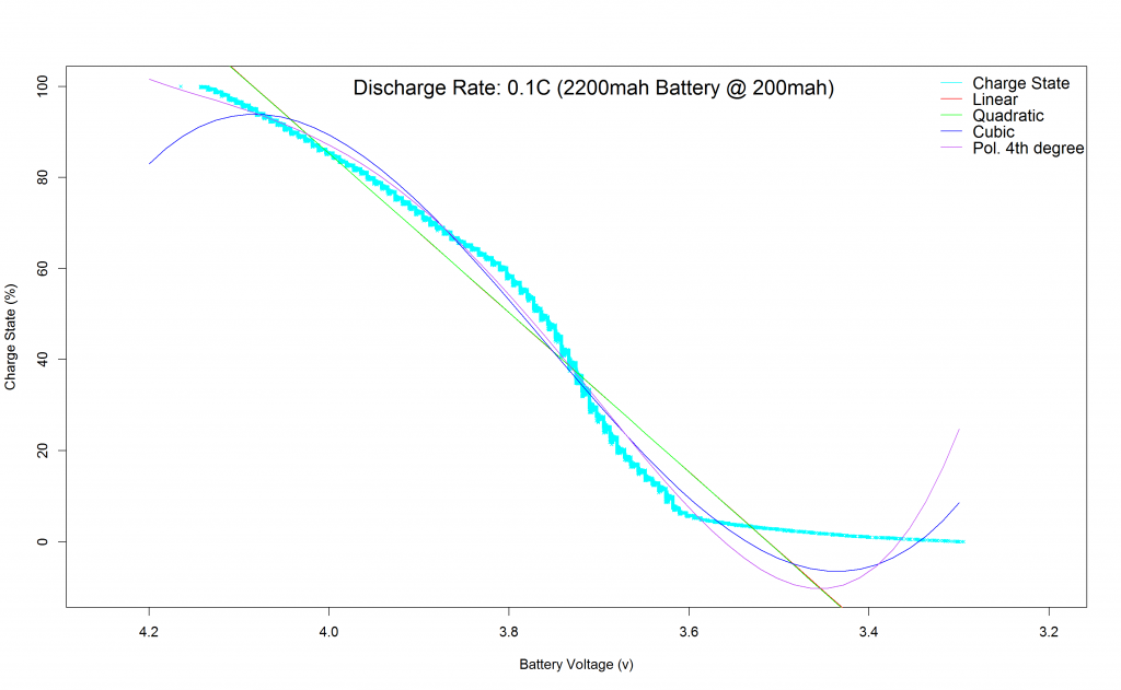
Resulting polynomials matching the 200ma dicharge curve of  the 2200mah lipo battery:

The result was not as good as I expected, it seems lower degree polynomial functions aren’t able to fit the discharge curve nicely.

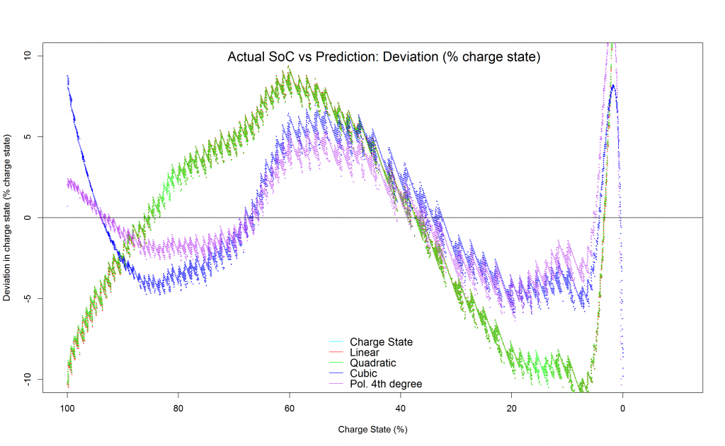
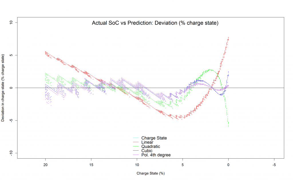
The deviation plot above shows how the fitting of a polynomial function up to the 4th degree results in a SoC estimation of more than +/-5% at times.

Splitting the data

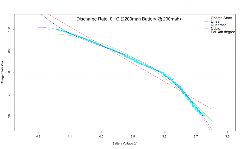
To get a better fit, the data will be split into two parts at 3.67 volts. This will allow for two polynomial equations to be fit to the two parts of the dataset. With that a much better fit was achived.

Polinomials of the first part of the dataset:

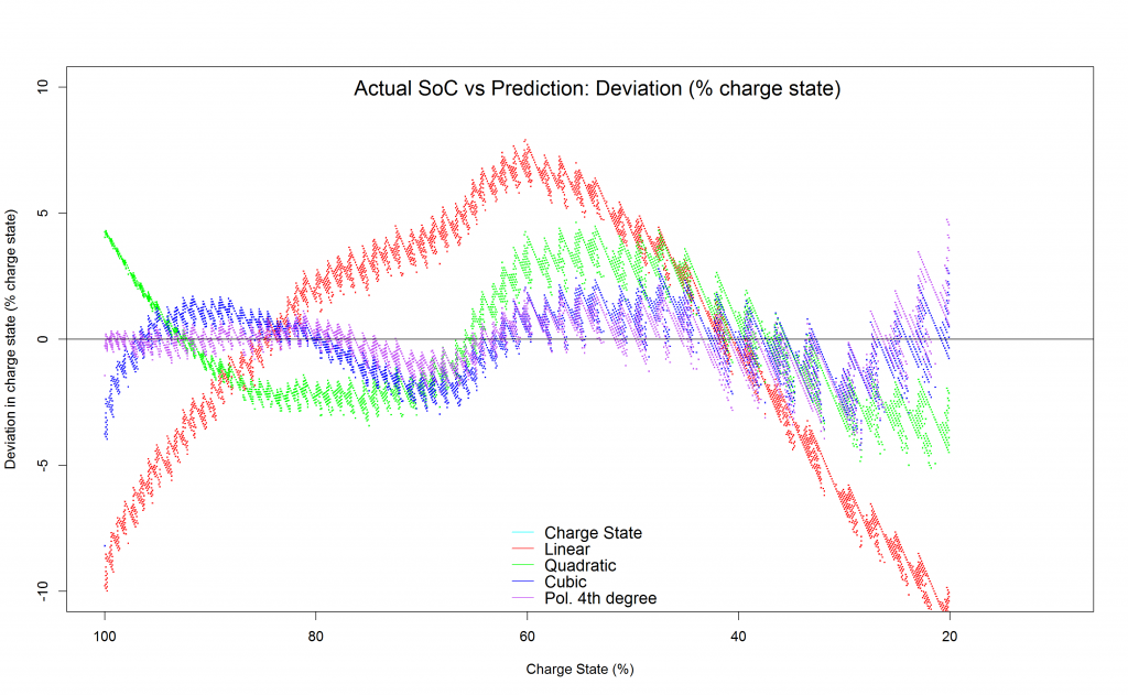
Deviations first part:

It seems quite a nice fit for the first part of the dataset was found using a Cubic polynomial function. State of Charge estimation deviation seems to be roughly between +/- 2.5%.

Polinomials of the second part of the dataset:

Deviations second part:

Again the cubic  fit does well with a roughly +/- 2% deviation in the State of Charge estimations.

Coefficients for the polynomial curves above (split dataset at 3.6v)

Part 1 for Battery Voltage >= 3.6v

> fit1
Coefficients:
(Intercept)            x  
     -590.7        169.1  
> fit2
Coefficients:
            (Intercept)  poly(x, 2, raw = TRUE)1  poly(x, 2, raw = TRUE)2  
                -5078.9                   2482.2                   -297.6  
> fit3 
Coefficients:
            (Intercept)  poly(x, 3, raw = TRUE)1  poly(x, 3, raw = TRUE)2  poly(x, 3, raw = TRUE)3  
                 -72167                    54226                   -13591                     1138  
> fit4
Coefficients:
            (Intercept)  poly(x, 4, raw = TRUE)1  poly(x, 4, raw = TRUE)2  poly(x, 4, raw = TRUE)3  poly(x, 4, raw = TRUE)4  
                -840650                   844356                  -318083                    53263  -3345  

Part 2 for Battery Voltage < 3.6v 

> fit1
Coefficients:
(Intercept)            x  
    -201.51        58.81  
> fit2
Coefficients:
            (Intercept)  poly(x, 2, raw = TRUE)1  poly(x, 2, raw = TRUE)2  
                 4017.7                  -2338.2                    340.1  
> fit3 
Coefficients:
            (Intercept)  poly(x, 3, raw = TRUE)1  poly(x, 3, raw = TRUE)2  poly(x, 3, raw = TRUE)3  
                 -67036                    58405                   -16959                     1641  
> fit4
Coefficients:
            (Intercept)  poly(x, 4, raw = TRUE)1  poly(x, 4, raw = TRUE)2  poly(x, 4, raw = TRUE)3  poly(x, 4, raw = TRUE)4  
                 484653                  -571501                   252624                   -49614  3653  

Resultung SOC formula

If v >= 3.6 Then
SOC = -72167 + 54226*v – 13591*v^2 + 1138*v^3
Else
SOC = -67036 + 58405*v – 16959*v^2 + 1641*v^3
EndIf

Conclusion